R Online Editor - Free Statistical Computing & Data Analysis Tool 2025

Statistical analysis shouldn't require complex software installations. Running R locally means downloading gigabytes, managing packages, and troubleshooting environment issues—blocking quick data exploration and learning.

This guide shows how to run R programming online instantly using browser-based execution with WebR (R 4.4+). Learn statistical computing, create data visualizations, and perform hypothesis testing with real-time output—no installations or configurations required.

Table of Contents

1. What is R Programming
2. Why Use R Programming
3. Why Use tools-online.app R Editor
4. How to Run R Code Online: Step-by-Step
5. Fixing Common R Errors
6. R Programming Templates and Examples
7. R Programming Best Practices
8. Related Data Science Tools

What is R Programming

R is a programming language and software environment for statistical computing, data analysis, and graphics. Developed by statisticians for statisticians, R provides comprehensive tools for data manipulation, statistical modeling, and visualization.

R excels at handling complex statistical operations, from basic descriptive statistics to advanced machine learning algorithms. The language supports vectors, matrices, data frames, and lists as core data structures, making it ideal for mathematical and statistical computations.

Core R capabilities:

• Statistical analysis: T-tests, ANOVA, regression, correlation
• Data visualization: Plots, histograms, boxplots, scatter plots
• Data manipulation: Filtering, grouping, aggregation, transformation
• Programming constructs: Functions, loops, conditionals, packages
• Mathematical operations: Linear algebra, probability distributions

R is widely used in academia, research, finance, healthcare, and data science for its powerful statistical capabilities and extensive package ecosystem (CRAN repository with 18,000+ packages).

Why Use R Programming

R is the gold standard for statistical analysis, but local installation creates barriers. Online R editors remove friction for learning, teaching, and quick data exploration.

Challenges with Local R Installation

Traditional setup barriers:

• Large downloads - R + RStudio = 500MB+ installation
• Package management - Dependency conflicts, version mismatches
• Environment setup - Path configurations, library locations
• System requirements - Administrator access needed
• Updates - Manual R and package version management

According to data science education research, eliminating installation reduces time-to-first-analysis from 2+ hours to under 5 minutes.

Benefits of Online R Execution

Instant statistical analysis:

• Zero installation—works in any browser
• No configuration needed
• Consistent environment across devices
• Latest R version (4.4+) via WebR

Learning advantages:

• Focus on R syntax, not setup
• Try statistical examples immediately
• Share working code with students/colleagues
• Practice without breaking local environment

Quick data insights:

• Run statistical tests instantly
• Generate visualizations in seconds
• Explore datasets without imports
• Export results immediately

For database-driven analysis, see PostgreSQL Query Editor.

Why Use tools-online.app R Editor

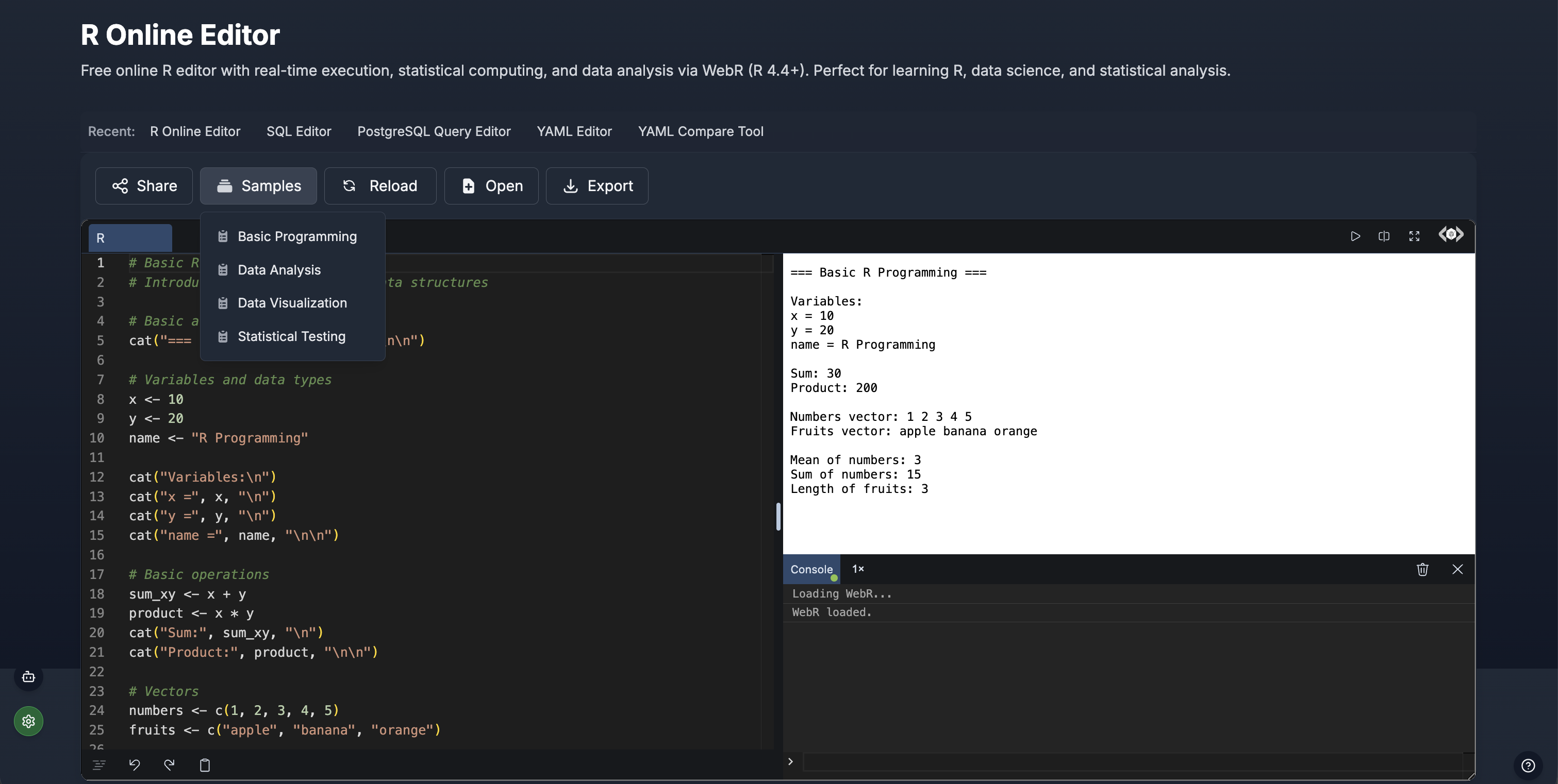
The R Editor on tools-online.app provides WebR-powered execution with syntax highlighting and real-time statistical output.

Key Features

Top Action Bar:

• Share - Generate shareable links with R code and results
• Samples - Load pre-written R examples (programming, analysis, visualization, testing)
• Reload - Reset editor and clear output
• Open - Upload R script files (.R, .r)
• Export - Download R code and statistical output

Editor Panel:

• Line numbers - Navigate code easily (1-25+ visible)
• Syntax highlighting - Color-coded comments (green), functions (orange), strings (orange quotes)
• WebR execution - Real-time R 4.4+ interpreter in browser
• Auto-completion - Statistical function suggestions as you type
• Error detection - Immediate feedback on syntax errors

Sample Templates:

• Basic Programming - Variables, data types, control structures
• Data Analysis - Descriptive statistics, data manipulation, aggregation
• Data Visualization - Plots, histograms, scatter plots, bar charts
• Statistical Testing - T-tests, ANOVA, correlation, regression analysis

How to Use AI for R Programming Tasks

Step 1: Configure AI (one-time setup)

1. Get your API key from AIML API
2. Click "Settings" icon(located lower left) in any tools-online.app tool.
   
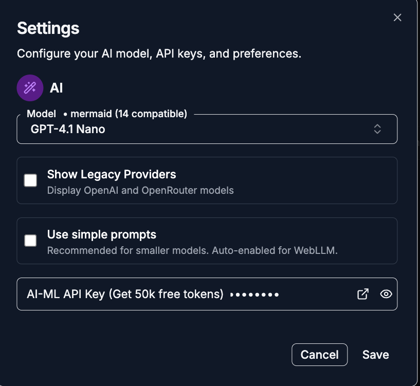
3. Add API key and save.
   

Step 2: Open AI Chat

1. Click the AI Chat button(located lower left)
   
2. Choose "Generate" mode and provide natural language descriptions:
   

AI Generation Examples:

• "Create R code to perform t-test comparing two groups"
• "Generate scatter plot with correlation analysis in R"
• "Write R script for linear regression with model diagnostics"
• "Create boxplots comparing multiple groups with statistical tests"
• "Generate R code for data cleaning and summary statistics"

AI Capabilities:

• Statistical Analysis - Generate code for t-tests, ANOVA, regression, correlation
• Data Visualization - Create plots, charts, and statistical graphics
• Data Manipulation - Filter, group, aggregate, and transform datasets
• Error Debugging - Analyze and fix R syntax and logic issues
• Code Optimization - Improve R script efficiency and readability

How to Run R Code Online: Step-by-Step

Method 1: Write R Code from Scratch

Step 1: Visit tools-online.app/tools/r

Step 2: Type R code in the editor panel

Example - basic statistical calculation:

# Basic statistical analysis
scores <- c(85, 92, 78, 95, 88, 76, 91, 84, 89, 93)

cat("Dataset Statistics:\n")
cat("Mean:", mean(scores), "\n")
cat("Median:", median(scores), "\n") 
cat("Standard Deviation:", sd(scores), "\n")
cat("Sample size:", length(scores), "\n")

Step 3: Click Run button (play icon)

Step 4: View statistical output in console:

Dataset Statistics:
Mean: 87.1 
Median: 88.5 
Standard Deviation: 6.348228 
Sample size: 10

Step 5: Modify parameters and re-run for different analyses

Method 2: Load Sample R Scripts

Step 1: Click Samples button

Step 2: Choose example category:

• Basic Programming - Variables, vectors, data structures
• Data Analysis - Statistics, aggregation, data frames
• Data Visualization - Plots, charts, graphics
• Statistical Testing - Hypothesis tests, regression models

Step 3: Example code loads with syntax highlighting

Step 4: Click Run to execute and see statistical results

Step 5: Modify parameters to explore different analyses

Method 3: Upload R Script Files

Step 1: Click Open button

Step 2: Select .R or .r file from computer

Step 3: File content loads into editor with line numbers

Step 4: Run complete script to execute all analyses

Step 5: Export results and modified code

Fixing Common R Errors

Understanding proper R syntax helps debug statistical programming issues quickly. Here's how to identify and fix frequent R problems:

Proper R Syntax Requirements

Valid R code must follow these rules:

1. Use proper assignment operators: <- or =
2. Match opening and closing parentheses/brackets
3. Quote character strings with single or double quotes
4. Use correct function syntax with parentheses
5. Separate function arguments with commas
6. End statements properly (semicolons optional)

Common Error Types and Solutions

1. Incorrect Assignment Operators

❌ Incorrect:

x = <- 10  # Mixed operators
y == 20    # Comparison instead of assignment

✅ Correct:

x <- 10    # Preferred assignment
y <- 20    # or y = 20

2. Missing or Unmatched Parentheses

❌ Incorrect:

mean(c(1, 2, 3, 4, 5)  # Missing closing parenthesis
plot(x, y))            # Extra closing parenthesis

✅ Correct:

mean(c(1, 2, 3, 4, 5))
plot(x, y)

3. Unquoted Character Strings

❌ Incorrect:

name <- John Doe       # Unquoted string
category <- Product A  # Space in unquoted string

✅ Correct:

name <- "John Doe"
category <- "Product A"

4. Incorrect Vector Creation

❌ Incorrect:

numbers <- [1, 2, 3, 4, 5]     # Wrong brackets
fruits <- ("apple", "banana")   # Wrong parentheses

✅ Correct:

numbers <- c(1, 2, 3, 4, 5)
fruits <- c("apple", "banana")

5. Object Name Errors

❌ Incorrect:

my.data <- data.frame(x = 1:5)
print(mydata)          # Wrong name (missing dot)

✅ Correct:

my.data <- data.frame(x = 1:5)
print(my.data)         # Exact name match

6. Function Argument Errors

❌ Incorrect:

plot(x y)              # Missing comma
mean(data na.rm=TRUE)  # Missing comma

✅ Correct:

plot(x, y)
mean(data, na.rm = TRUE)

Debugging Tips

• Check parentheses pairing by counting opening/closing
• Use syntax highlighting to spot unquoted strings
• Verify object names are spelled exactly as defined
• Test with small datasets before running complex analyses
• Use R's built-in help with ?function_name

R Programming Templates and Examples

Essential R operations for beginners:

Copy Basic Programming Template in R Editor

# Basic R Programming Example
cat("=== Basic R Programming ===\n\n")

# Variables and data types
x <- 10
y <- 20
name <- "R Programming"

cat("Variables:\n")
cat("x =", x, "\n")
cat("y =", y, "\n") 
cat("name =", name, "\n\n")

# Basic operations
sum_xy <- x + y
product <- x * y
cat("Sum:", sum_xy, "\n")
cat("Product:", product, "\n\n")

# Vectors
numbers <- c(1, 2, 3, 4, 5)
fruits <- c("apple", "banana", "orange")

cat("Vectors:\n")
print(numbers)
print(fruits)

Data Analysis Template

Statistical analysis and data manipulation:

# Sample dataset for analysis
scores <- c(85, 92, 78, 95, 88, 76, 91, 84, 89, 93)

# Descriptive statistics
cat("Descriptive Statistics:\n")
cat("Mean:", mean(scores), "\n")
cat("Median:", median(scores), "\n")
cat("SD:", sd(scores), "\n")
cat("Variance:", var(scores), "\n")
cat("Min:", min(scores), "\n") 
cat("Max:", max(scores), "\n")

# Quantiles
cat("\nQuantiles:\n")
print(quantile(scores))

# Data frame operations
df <- data.frame(
  name = c("Alice", "Bob", "Charlie"),
  age = c(25, 30, 35),
  score = c(85, 92, 78)
)

cat("\nData Frame:\n")
print(df)
cat("Average age:", mean(df$age), "\n")

Copy Data Analysis Template in R Editor

Data Visualization Template

Copy Data Visualization Template in R Editor

Creating plots and statistical graphics:

# Sample data for visualization
x <- 1:10
y <- x^2

# Scatter plot
plot(x, y,
     main = "Quadratic Relationship",
     xlab = "X Values", 
     ylab = "Y Values",
     pch = 19,
     col = "blue")

# Add trend line  
lines(x, y, col = "red", lwd = 2)

# Histogram of random data
data <- rnorm(1000, mean = 100, sd = 15)

hist(data,
     main = "Normal Distribution",
     xlab = "Values",
     ylab = "Frequency", 
     col = "lightblue",
     breaks = 30)

Statistical Testing Template

Copy Statistical Testing Template in R Editor

Hypothesis testing and statistical inference:

# Sample data for two groups
group_a <- c(78, 82, 85, 79, 88, 92, 76, 84)
group_b <- c(85, 89, 91, 87, 93, 95, 88, 90)

# Descriptive statistics by group
cat("Group A - Mean:", mean(group_a), "SD:", sd(group_a), "\n")
cat("Group B - Mean:", mean(group_b), "SD:", sd(group_b), "\n\n")

# Two-sample t-test
t_result <- t.test(group_a, group_b)
cat("T-test Results:\n")
print(t_result)

# Correlation analysis
correlation <- cor(group_a[1:length(group_b)], group_b)
cat("\nCorrelation:", correlation, "\n")

R Programming Best Practices

1. Use Clear Variable Names

Why: Improves code readability and debugging

Best Practice:

# Good: Descriptive names
student_scores <- c(85, 92, 78, 95, 88)
average_score <- mean(student_scores)

# Avoid: Unclear abbreviations
ss <- c(85, 92, 78, 95, 88)
as <- mean(ss)

2. Comment Your Statistical Analysis

Why: Explains methodology and assumptions

Implementation:

# Perform two-sample t-test to compare groups
# Assumptions: Normal distribution, equal variances
# H0: No difference in means between groups
# H1: Significant difference exists (two-tailed)
t_result <- t.test(group_a, group_b, var.equal = TRUE)
cat("p-value:", t_result$p.value, "\n")

# Interpret results
if(t_result$p.value < 0.05) {
  cat("Reject H0: Groups are significantly different\n")
} else {
  cat("Fail to reject H0: No significant difference\n")
}

3. Structure Data Analysis Workflow

Why: Organized approach improves reproducibility

Standard workflow:

# 1. Data loading and exploration
data <- read.csv("dataset.csv")
cat("Dataset dimensions:", dim(data), "\n")
summary(data)

# 2. Data cleaning
data_clean <- data[complete.cases(data), ]  # Remove missing values
outliers <- which(abs(scale(data_clean$value)) > 3)  # Identify outliers

# 3. Descriptive statistics
cat("Mean:", mean(data_clean$value), "\n")
cat("SD:", sd(data_clean$value), "\n")

# 4. Statistical testing
# 5. Visualization
# 6. Interpretation

4. Validate Statistical Assumptions

Why: Ensures appropriate test selection and valid results

Example:

# Check normality assumption for t-test
shapiro_test <- shapiro.test(group_a)
cat("Normality test p-value:", shapiro_test$p.value, "\n")

# Check equal variances
var_test <- var.test(group_a, group_b)
cat("Equal variances test p-value:", var_test$p.value, "\n")

# Choose appropriate test based on assumptions
if(shapiro_test$p.value > 0.05 & var_test$p.value > 0.05) {
  # Use standard t-test
  result <- t.test(group_a, group_b, var.equal = TRUE)
} else {
  # Use Welch's t-test or non-parametric alternative
  result <- t.test(group_a, group_b, var.equal = FALSE)
}

5. Handle Missing Data Appropriately

Why: Missing data affects statistical power and validity

Strategies:

# Check for missing data
missing_count <- sum(is.na(data))
cat("Missing values:", missing_count, "\n")

# Complete case analysis
complete_data <- data[complete.cases(data), ]

# Mean imputation (use cautiously)
data$value[is.na(data$value)] <- mean(data$value, na.rm = TRUE)

# List-wise deletion for specific functions
correlation <- cor(data$x, data$y, use = "complete.obs")

6. Use Vectorized Operations

Why: Faster execution and cleaner code

Efficient approach:

# Good: Vectorized operations
scores <- c(85, 92, 78, 95, 88)
standardized <- (scores - mean(scores)) / sd(scores)

# Avoid: Loops for simple operations  
standardized <- numeric(length(scores))
for(i in 1:length(scores)) {
  standardized[i] <- (scores[i] - mean(scores)) / sd(scores)
}

7. Save and Export Results

Why: Preserve analysis outputs for reporting

Best practices:

# Save statistical test results
results <- list(
  descriptive = summary(data),
  t_test = t.test(group_a, group_b),
  correlation = cor.test(x, y)
)

# Export visualizations
png("analysis_plot.png", width = 800, height = 600)
plot(x, y, main = "Analysis Results")
dev.off()

# Export data summaries
write.csv(summary_stats, "summary_statistics.csv")

8. Test Code with Sample Data

Why: Verify analysis works before applying to real datasets

Approach:

# Create test data with known properties
set.seed(123)  # Reproducible results
test_data <- rnorm(100, mean = 50, sd = 10)

# Run analysis on test data
test_mean <- mean(test_data)
cat("Test mean (should be ≈ 50):", test_mean, "\n")

# If test passes, apply to real data
real_analysis <- mean(actual_data)

Related Tools

Data Tools:

• PostgreSQL Editor - Database queries for large datasets
• SQL Editor - Lightweight data analysis with SQLite

Dataset Management:

• Data Compare Tool - Compare Excel/CSV datasets with statistical summaries
• JSON Tool - Validate JSON data exports from R analyses
• YAML Tool - Format configuration files for R environments

Complete Tool Collections

Browse by Category:

• Online Data Tools - Complete statistical and data analysis toolkit
• Online Code Tools - Programming environment with 15+ languages
• Online Compare Tools - Data and code comparison suite
• Online Productivity Tools - Research workflow optimization

Resources

• R Documentation - Official R language reference
• CRAN Task Views - R packages by statistical domain
• R for Data Science - Comprehensive R programming guide
• Statistical Computing with R - Advanced statistical methods

Discover More: Visit tools-online.app to explore our complete suite of statistical computing and data analysis tools.